Appendix B: Information Geometry and Logarithmic Metric

In Volume IV “The Logarithmic Eye” of Vector Cosmology III, we explored how living organisms decode the exponentially exploding cosmic information through logarithmic operations (Weber-Fechner Law). This physiological mechanism is not an evolutionary accident, but is based on deeper mathematical principles—Information Geometry.

This appendix will show that logarithmic perception is actually the natural distance metric on a Statistical Manifold. Just as the FS metric defines the distance between quantum states, the Fisher information metric defines the distance between probability distributions. Our senses are essentially measuring geometric arc lengths in signal space.

B.1 From Hilbert Space to Statistical Manifold

In the first book of this series, we introduced the Fubini-Study (FS) Metric, which is the natural geometry describing changes in pure-state quantum vectors $|\psi ⟩$.

But at the macroscopic level, biological senses typically process not pure states, but mixed states or classical probability distributions $p(x|\theta )$ (e.g., Poisson distribution of photons reaching the retina, where $\theta$ is light intensity).

These probability distributions form a curved geometric space called a Statistical Manifold.

• Each point on the manifold represents a specific probability distribution.

• The changes we perceive (such as brightness increasing) correspond to displacements on the manifold.

B.2 Fisher Information Metric

On this classical statistical manifold, the unique natural Riemannian metric measuring the “distinguishability” between two points is the Fisher Information Metric, denoted $g_{ij}$.

For a family of probability distributions $p(x|\theta )$ described by parameter $\theta$, the metric tensor is defined as:

$$g_{\theta \theta }=\int p(x|\theta ){\left(\frac{\partial \ln p(x|\theta )}{\partial \theta }\right)}^{2}dx$$

The physical meaning of this formula is: The intensity of change in the probability distribution $p(x)$ when we slightly adjust parameter $\theta$ (external stimulus).

• If the change is intense (large information), the distance is long, and we can easily distinguish.

• If the change is tiny (small information), the distance is short, and we have difficulty distinguishing.

B.3 Geometric Derivation of Weber-Fechner Law

Now, we apply this geometric framework to the sensory system.

Assume the external stimulus intensity is $I$ (e.g., light intensity). Signals received by the senses are typically affected by multiplicative noise (because $I$ is an energy scale with non-negativity and scale invariance).

This corresponds to the Scale Family distribution in statistics, with the form:

$$p(x|I)=\frac{1}{I}f\left(\frac{x}{I}\right)$$

Let us calculate the Fisher information metric $g_{II}$ for this distribution:

Substituting into the definition formula and performing integration (omitting intermediate steps), for scale families, the metric tensor always takes the form:

$$g_{II}=\frac{C}{I^2}$$

where $C$ is a constant related to the distribution shape.

Thus, the infinitesimal geometric distance $ds$ in signal space is:

$$ds=\sqrt{g_{II}}dI=\sqrt{C}\frac{dI}{I}$$

This directly leads to Weber’s Law: The just noticeable difference (threshold of geometric distance $ds$) is inversely proportional to stimulus intensity $I$.

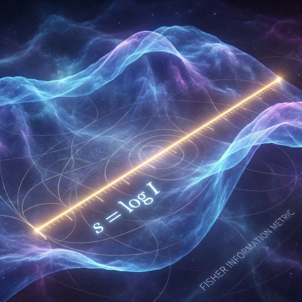
Integrating the above equation, we obtain the macroscopic sensation magnitude $S$ (i.e., the total geometric distance from reference point $I_0$ to $I$):

$$S={\int }_{I_0}^{I}ds=\sqrt{C}{\int }_{I_0}^I\frac{dI}{I}=k\ln \left(\frac{I}{I_0}\right)$$

This is Fechner’s Law $S=k\ln I$.

B.4 Sensation as Geodesic

This derivation proves: Biological sensation intensity is strictly equal to the geodesic length of the signal in information geometric space.

• The FS Metric governs microscopic quantum evolution ($v_{ext}^2+v_{int}^2=c_{FS}^2$).

• The Fisher Metric governs macroscopic sensory cognition ($S\propto \ln I$).

The two are isomorphic in mathematical structure. This again confirms the core view of the entire book: Life is an isomorphic mapping of the universe’s geometric structure. The reason we perceive the world as logarithmic is because our brains, unconsciously, are constantly performing extremely precise information geometric measurements.