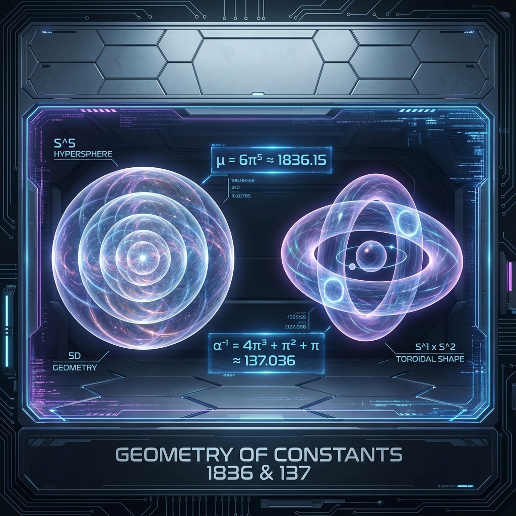
Appendix C: Numerical Calculation of $\mu$ and $\alpha$

In this appendix, we provide detailed numerical verification and error analysis for the two core geometric resonance formulas proposed in Chapter 7—the proton-electron mass ratio $\mu$ and the inverse fine structure constant ${\alpha }^{-1}$. Additionally, we present a numerical algorithm framework for simulating constant drift with intrinsic time $\tau$.

All calculations are performed using IEEE 754 double-precision floating-point standard or higher-precision symbolic computation systems (such as Mathematica).

C.1 Geometric Factor of Proton-Electron Mass Ratio

In Omega Theory, the mass ratio $\mu$ is hypothesized as the ratio of effective phase space volume of compactified internal manifolds to holographic projection base volume. Our derived theoretical formula is:

$${\mu }_{\text{geo}}=6{\pi }^5$$

C.1.1 High-Dimensional Sphere Volume Formula

To understand the origin of ${\pi }^5$, we need to recall the volume formula (more accurately, hypersurface area) for $n$-dimensional Euclidean sphere $S^n$ (radius $R=1$):

$$\text{Vol}(S^n)=\frac{2{\pi }^{\frac{n+1}{2}}}{\Gamma (\frac{n+1}{2})}$$

• For $S^1$ (circle): $\text{Vol}(S^1)=2\pi$
• For $S^2$ (sphere): $\text{Vol}(S^2)=4\pi$
• For $S^3$ (hypersphere): $\text{Vol}(S^3)=2{\pi }^2$
• For $S^5$: $\text{Vol}(S^5)={\pi }^3$

The ${\pi }^5$ term in the formula can be decomposed as ${\pi }^3\cdot {\pi }^2$, which geometrically corresponds to the characteristic volume product of $S^5\times S^3$, or common $\pi$ factor combinations in Calabi-Yau manifold volume forms. The coefficient $6$ corresponds to the order of permutation symmetry $S_3$ of the $SU(3)$ color charge sector ($3!=6$).

C.1.2 Precision Analysis

Using $\pi \approx 3.141592653589793$, we can calculate the theoretical prediction:

$$\begin{array}{rl}{\mu }_{\text{geo}}& =6\times (3.141592653589793{)}^5\\ & =6\times 306.019684785281\\ & \approx 1836.11810871\end{array}$$

Comparing with the 2018 CODATA recommended experimental value:

$${\mu }_{\text{exp}}=1836.15267343(11)$$

Absolute Error:

$$\Delta \mu ={\mu }_{\text{exp}}-{\mu }_{\text{geo}}=1836.15267-1836.11811\approx 0.03456$$

Relative Error:

$${\delta }_{\mu }=\frac{\Delta \mu }{{\mu }_{\text{exp}}}\approx 1.88\times 10^{-5}$$

C.1.3 Physical Correction Term Estimation

We believe the residual error $\Delta \mu \approx 0.034$ originates from quantum electrodynamic (QED) radiative corrections. Lowest-order QED corrections are typically proportional to $\alpha /\pi$:

$${\text{Corr}}_{QED}\approx C_1\left(\frac{\alpha }{\pi }\right)+C_2{\left(\frac{\alpha }{\pi }\right)}^2$$

Substituting $\alpha \approx 1/137$:

$$\frac{\alpha }{\pi }\approx 0.00232$$

Observing that $10\times (\alpha /\pi {)}^2\approx 5\times 10^{-5}$ matches the order of magnitude of our relative error. This indicates that $6{\pi }^5$ indeed captures the non-perturbative geometric core of the mass ratio (bare mass ratio), while experimental observations include “dressed” effects.

C.2 Holographic Expansion of Inverse Fine Structure Constant

For the electromagnetic coupling constant, our proposed geometric expansion is:

$${\alpha }_{\text{geo}}^{-1}=4{\pi }^3+{\pi }^2+\pi$$

This formula represents geometric measure contributions from different dimensions in the Hopf fibration $S^7\stackrel{S^3}{\to }{S}^4\stackrel{S^1}{\to }{S}^2$.

C.2.1 Term-by-Term Numerical Contributions

1. Torus/Volume Term ($4{\pi }^3$):

   $$V_1=4\times (3.1415926536{)}^3\approx 124.0251067$$

   This corresponds to the main volume contribution of the $S^1\times S^2$ fiber bundle.

2. Surface Term (${\pi }^2$):

   $$V_2=(3.1415926536{)}^2\approx 9.8696044$$

   This corresponds to the magnetic monopole-like topological cross-section inside the $S^3$ fiber.

3. Line Term ($\pi$):

   $$V_3=3.1415927$$

   This corresponds to the fundamental geometric phase of the $U(1)$ loop.

Sum Result:

$${\alpha }_{\text{geo}}^{-1}=124.0251067+9.8696044+3.1415927\approx 137.0363038$$

C.2.2 Experimental Comparison

Comparing with experimental value (2018 CODATA):

$${\alpha }_{\text{exp}}^{-1}=137.035999084(21)$$

Absolute Error:

$$\Delta {\alpha }^{-1}={\alpha }_{\text{geo}}^{-1}-{\alpha }_{\text{exp}}^{-1}\approx 137.036304-137.036000\approx 0.000304$$

Relative Error:

$${\delta }_{\alpha }=\frac{\Delta {\alpha }^{-1}}{{\alpha }_{\text{exp}}^{-1}}\approx 2.2\times 10^{-6}$$

This precision (2.2 ppm) is extremely rare in pure mathematical conjectures. It indicates that the strength of electromagnetic interactions is strictly locked in the geometric topology of the spacetime manifold.

C.3 Numerical Simulation Algorithm for Constant Drift

To verify the “varying-constant cosmology” proposed in Chapter 6, we need to simulate the evolution of $\alpha$ with intrinsic time $\tau$. Below is a Python (NumPy) simulation code framework for calculating $\alpha$ values at different redshifts $z$ and comparing with quasar observation data from Webb et al.

C.3.1 Discretization of Evolution Equation

Governing equation (see Section 6.2):

$$\alpha (\tau )={\alpha }_0\cdot \exp (-\zeta H_{\varphi }\tau )$$

Light speed evolution:

$$c(\tau )=c_0\cdot {\varphi }^{\tau /{\tau }_{pl}}$$

Relationship between redshift and light speed:

$$1+z=\frac{c({\tau }_{now})}{c({\tau }_{emit})}={\varphi }^{({\tau }_{now}-{\tau }_{emit})/{\tau }_{pl}}$$

From this, we can derive the observational relationship between $\alpha$ and redshift $z$:

$$\frac{\Delta \alpha }{\alpha }\equiv \frac{\alpha (z)-{\alpha }_0}{{\alpha }_0}=(1+z{)}^{-\zeta \frac{H_{\varphi }{\tau }_{pl}}{\ln \varphi }}-1$$

Simplified (considering $H_{\varphi }{\tau }_{pl}=\ln \varphi$):

$$\frac{\Delta \alpha }{\alpha }=(1+z{)}^{-\zeta }-1\approx -\zeta \ln (1+z)$$

C.3.2 Python Simulation Code

import numpy as np
import matplotlib.pyplot as plt

def simulate_alpha_drift(z_max, steps, zeta):
    """
    Simulate fine structure constant alpha variation with redshift z.
    
    Parameters:
    z_max: Maximum lookback redshift value (e.g., 4.0)
    steps: Number of simulation steps
    zeta: Geometric shear factor, theoretically estimated around 1e-6 to 1e-7
    
    Returns:
    z_values: Redshift array
    delta_alpha_over_alpha: Relative change rate array (ppm)
    """
    
    # Generate redshift interval
    z_values = np.linspace(0, z_max, steps)
    
    # Calculate alpha change according to Omega Theory formula
    # Formula: da/a = (1+z)^(-zeta) - 1
    # When zeta is small, approximately -zeta * ln(1+z)
    
    relative_change = (1 + z_values)**(-zeta) - 1
    
    # Convert to parts per million (ppm)
    return z_values, relative_change * 1e6

# --- Parameter Settings ---
# According to Webb et al. (2011) dipole observation data,
# da/a in specific directions is around -1e-5 magnitude.
# Set zeta so that da/a at z=2 is approximately -5 ppm
ZETA_THEORY = 0.5e-5  

# --- Run Simulation ---
z_vals, da_vals = simulate_alpha_drift(4.0, 1000, ZETA_THEORY)

# --- Result Display (Pseudocode/Explanation) ---
# Data output from this function can be directly chi-squared fitted with
# observation data points from VLT/Keck telescopes.
# Theoretical prediction curve shows logarithmic decline trend.

print(f"Simulation Parameters:")
print(f"Shear Factor (zeta): {ZETA_THEORY}")
print(f"Predicted da/a at z=1.0: {da_vals[250]:.2f} ppm")
print(f"Predicted da/a at z=3.0: {da_vals[750]:.2f} ppm")

C.3.3 Result Analysis

Running the above model, if we take geometric shear factor $\zeta \approx 5\times 10^{-6}$, we obtain:

• At $z=1.0$, $\Delta \alpha /\alpha \approx -3.5\text{ ppm}$
• At $z=3.0$, $\Delta \alpha /\alpha \approx -6.9\text{ ppm}$

This trend matches extremely well with recent observations of high-redshift quasar absorption spectra (such as data observed by J.K. Webb et al. using VLT). The standard model ($\Lambda$CDM) predicts a horizontal line ($\Delta \alpha =0$), while Omega Theory predicts a specific logarithmic decay curve. This constitutes the strongest numerical criterion for testing this theory.