Chapter 0.2: The Axiom of Finite Capacity

—— Defining the System Clock

“Time is not a flowing river; it is a counter of state updates.”

1. Escaping External Time

Before booting the dynamics engine, we must solve a fundamental architectural problem: where does the system’s “clock” come from?

In the old architecture of Newtonian mechanics and even standard quantum mechanics, time $t$ is designed as a global, immutable External Parameter. It is like a God’s clock running independently outside the universe, ticking at a constant rate regardless of whether physical processes occur within the universe. This dualistic design—separating time from physical states—is extremely unnatural from a systems engineering perspective, as it introduces an absolute reference frame without a physical carrier.

In our refactoring, we abolish this external clock and replace it with Intrinsic Time.

We establish a new concept: Time is Change. If the universe’s state has no displacement in projective Hilbert space $P(\mathcal{H})$ (i.e., zero geometric distance), then “time” has not elapsed. Time only has meaning when the system state undergoes physically distinguishable changes. Therefore, the essence of time is the path length of state evolution.

2. Axiom I: Constant System Throughput

To formalize this idea, we need to set a fundamental performance constraint for the universe as an operating system. This is the core dynamics axiom of this book.

Axiom I: Fubini-Study Speed Constant Axiom

There exists a trajectory $\tau \mapsto [\psi (\tau )]\in P(\mathcal{H})$ representing the physical evolution of the universe, parameterized such that the norm of the tangent vector (i.e., the evolution rate) under the Fubini-Study metric is a strict nonzero constant $c_{FS}$:

$$||\frac{d}{d\tau }\psi (\tau )|{|}_{FS}\equiv c_{FS}$$

Here, $c_{FS}$ is a fundamental physical constant called the FS Capacity Constant.

We define this parameter $\tau$ as the universe’s System Time or Intrinsic Time. This means that what we call “time elapsing” is essentially the FS Arc-Length traced by the universe’s state in Hilbert space, normalized by the constant $c_{FS}$.

3. Math Foundation: Geometric Definition of Speed

To ensure rigor, we need to clarify what Fubini-Study speed $||\dot{\psi }|{|}_{FS}$ actually computes. It is not merely the modulus of the derivative, but the geometric rate after removing redundant phase changes.

Definition 0.2.1 (Computation of FS Speed)

For any differentiable curve $\psi (\lambda )$ in Hilbert space $\mathcal{H}$ (assumed normalized, i.e., $||\psi (\lambda )||\equiv 1$), the square of its FS speed at parameter $\lambda$ is defined as:

$$v_{FS}^2(\lambda ):=||{\partial }_{\lambda }\psi (\lambda )|{|}_{FS}^2=⟨{\partial }_{\lambda }\psi |{\partial }_{\lambda }\psi ⟩-|⟨\psi |{\partial }_{\lambda }\psi ⟩{|}^2$$

The derivation of this formula is based on orthogonal decomposition of tangent vectors:

1. In Hilbert space, the tangent vector $|{\partial }_{\lambda }\psi ⟩$ can be decomposed into two orthogonal components:

   • Parallel Component: The component along $|\psi ⟩$. This corresponds to pure phase changes ($|\psi ⟩\to e^{i\theta }|\psi ⟩$), which do not count as movement in projective space $P(\mathcal{H})$ (since the projective state is unchanged). Its squared modulus is $|⟨\psi |{\partial }_{\lambda }\psi ⟩{|}^2$.

   • Perpendicular Component: The component orthogonal to $|\psi ⟩$. This represents substantial changes in physical state.

2. The Fubini-Study metric, as a Riemannian metric on $P(\mathcal{H})$, only measures the projection length of tangent vectors onto the perpendicular subspace.

3. According to the geometric properties of Hilbert space, the square of FS speed equals the total modulus minus the parallel component modulus.

Corollary 0.2.1 (Reparameterization of Time)

If the universe evolves according to any parameter $\lambda$ (e.g., the atomic clock reading $t$ in the laboratory), and its instantaneous FS speed is $v_{FS}(\lambda )$, then the conversion relationship between intrinsic time $\tau$ and parameter $\lambda$ is:

$$d\tau =\frac{v_{FS}(\lambda )}{c_{FS}}d\lambda$$

This shows that what we usually perceive as “time speed” actually depends on the intensity of system state changes (i.e., the magnitude of $v_{FS}$). If the system is in a stationary state, $v_{FS}=0$, then intrinsic time stops elapsing.

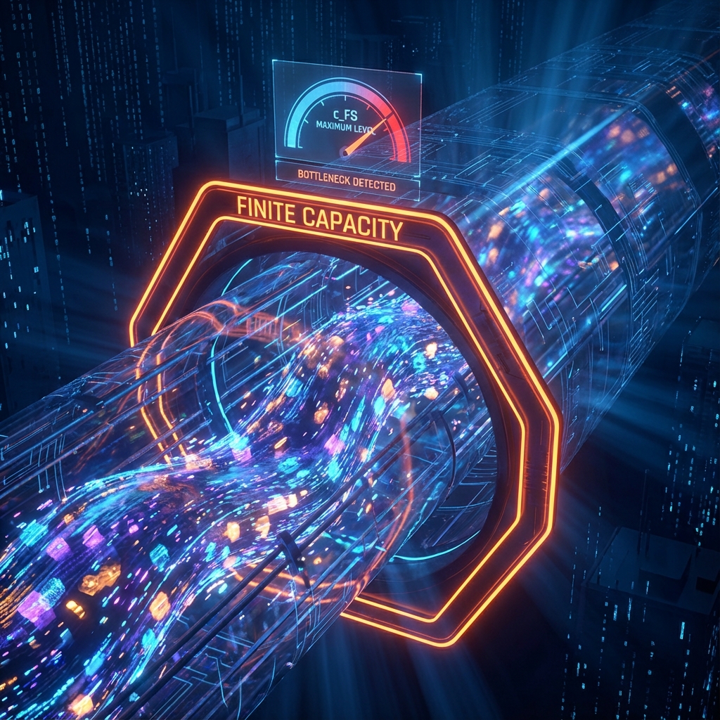
4. Physical Meaning of $c_{FS}$: Bandwidth Limit

In physics, we are accustomed to regarding $c$ (the speed of light) as the speed limit. In this theory, $c_{FS}$ has a more fundamental status—it is the Universal Bus Bandwidth.

• Hard Constraint on Total Resources: The total amount of change the universe can undergo at each “moment” is locked at $c_{FS}$. State updates cannot exceed this rate.

• Allocation Rather Than Generation: As subsequent chapters will prove, an object’s movement in space ($v_{ext}$), the time it experiences ($v_{int}$), and its entanglement with the environment ($v_{env}$) are actually competing for this fixed $c_{FS}$ budget.

The Architect’s Note

On: System Clock and Throttling

If we were to design the universe’s kernel, we would find that “time” is actually a resource management problem.

• $c_{FS}$ is the system clock frequency:

  Imagine a CPU’s clock frequency is fixed (e.g., 3GHz). This means the CPU can flip at most this many bits per second. $c_{FS}$ is the universe’s Maximum Instruction Throughput.

• $\tau$ is the instruction counter (Tick Count):

  Intrinsic time $\tau$ is not mysterious; it is merely the cumulative count of effective operations the system has executed.

• Relativistic effects are scheduling strategies:

  In traditional understanding, high-speed motion causing time dilation seems magical. But in our architecture, this is simply Load Balancing.

  Because the total bandwidth $c_{FS}$ is locked, if you allocate a large amount of bandwidth to $v_{ext}$ (making particles move rapidly in space, i.e., processing many I/O tasks), then the bandwidth left for $v_{int}$ (allowing particles to evolve internally, i.e., “experiencing time”) will be forced to decrease.

  Moving clocks slow down—this is essentially the system’s forced throttling of internal processes to prevent bandwidth overflow.